A lot has happened since my previous post, but I'd like to focus on the progress of SAE-ception. For those unfamiliar, SAE-ception is my attempt to leverage post-hoc interpretability tools during model training to encourage the model to learn more interpretable representations, and ideally become more monosemantic. This work was extended beyond that previos blog post into a paper, which was recently accepted into the Mechanistic Interpretability Workshop at NeurIPS. Below, I'll talk a little bit about where SAE-ception currently stands.
Background
Before diving into the results from the paper (which extended the MNIST digit work to CIFAR10 and ImageNet-1k), I'd like to spend a little bit of time going over what SAE-ception is and why we might expect it to work. For those unfamiliar with what I'm talking about here, I strongly recommend a skim of my my previous post, particularly for terminology used below.
SAE-ception is a novel technique that uses a sparse autoencoder (SAE) "in-the-loop" to guide the model towards more interpretable representations. Already, you probably have a few questions - what do you mean "in-the-loop"? How can an SAE be useful in this situation? What is the guidance you speak of and how does it work?
Well, let's start breaking this down one question at a time. By "in-the-loop", I mean that we apply the SAE during model training (note: when I say model training, I'm also including fine-tuning, perhaps this is a bit loose, but this is a blog after all).
This naturally leads us to the second question, as it probably isn't straightforward as to how an SAE can be helpful during model training, after all SAEs are primarily used for interpretability.
It comes back to the pigeonhole principle. Recall: the pigeonhole principle states that if more items (pigeons) are put into fewer containers (pigeonholes), then at least one container must contain more than one item. In the model itself, capacity is severely limited, meaning that the many semantic concepts our data contains must be overloaded into the nodes at each layer of the network, as we have far too few nodes compared to concepts (this phenomena has a fancy name: polysemanticity).
So, the motivating thought behind SAE-ception is the following: what if a lot of these pigeons don't matter? What if we have many "bad" pigeons that actually confuse and clutter our representations? More explicitly, there exists a slider with interpretability on one end and performance on the other. There should be a number of pigeons that allows us to optimize for the situation where we desire both: a model that is quite performant (perhaps not SOTA) and highly interpretable.
This might sound fine and dandy, but it probably still isn't clear how the SAE helps us find the optimal number of pigeons. Well, an SAE utilizes sparsity as a proxy for interpretability - it provides additional containers for our pigeons, ideally separating them in as close to a one pigeon to one container ratio. So, in the sparse space of an SAE we should have more clarity on what pigeons are actually present. Furthermore, since each container will have an activation, we can think of this as a score defining how important the pigeon is for the current task. This means we can select for the most important pigeons to the particular input and zero out (i.e. eliminate) the other, "bad" pigeons. Thus, our SAE can then decode this vector of only "good" pigeons and provide us with a target vector of what a more interpretable, but also performant, representation should look like at that layer.
One note to make here: when trimming these features, we probably want to do it as the class level. That is, keep the top-k features for a class active and turn off all other features, even if one of the top-k features is not active for a particular example of that class. We can find these features ("good" pigeons) by taking the average top-k sparse activations for that class. This is labeled as "feature sharpening" in the blog and paper.
From this point, we can use this target vector as the ground truth for auxiliary loss at that layer. We are telling the network that in addition to optimizing for the correct answer (this is the model's original loss function), please also spend some thought on trying to mimic this target vector at the specific layer we applied our SAE to (i.e. also optimize that layer's representation to be more interpretable). Also, since feature sharpening is dynamic (in the sense of unique to each class), we shouldn't really be removing any pigeons during this process, but more so optimizing each representation for its respective version of "good" pigeons. The only time we may see an extinction of a particular pigeon is if it was never really used by any class in the dataset (naively, this seems like a good outcome, though I'm sure there could be an adversarial or robustness counter-arguement).
We can also perform this process iteratively, spending X epochs training the model before training a fresh SAE to repeat the process above. This might be done to potentially account for feature drift (seems wise to adjust the target vector as our representations improve), or for fine-tuning towards a new dataset.
In short, SAE-ception uses an SAE to help identify candidate pigeons that are not useful to a particular input, trim these "bad" pigeons during decoder reconstruction, and use this resulting target vector to encourage the model to learn better representations in addition to maintaining its performance.
For visual learners, please see a copy of the two diagrams from the paper below. The Feature Sharpening Pipeline describes how we trim "bad" pigeons from a particular input. The SAE-ception training loop shows how we can perform this process iteratively.
An illustration of the Feature Sharpening pipeline. The process begins with the extracted polysemantic activation vector, , where mixed colors in each node represent multiple features. Our SAE encoder maps to a sparse vector , composed of largely monosemantic features (single colors) and inactive features (white). A Sharpen step then prunes less active features to create a sharpened vector (e.g., the cyan and orange features are removed). This sharpened vector is passed to the SAE decoder, which generates the final target, . The resulting reconstruction shows reduced polysemanticity, demonstrating the effect of the sharpening process.
The SAE-ception Training Loop. Top: First, the frozen model, , is used to generate a sharpened reconstructed target, , from an internal activation . Bottom: The new model, , is then trained. A total loss, , is computed by combining the standard task loss, , with an auxiliary loss, , that steers the new activation, , to match the sharpened target . This total loss is used to update the weights of during backpropagation.
Does SAE-ception work?
Preface: SAE-ception is still in its early stages. It's only been tested on a shallow MLP performing digit classificaiton on MNIST, a vision transformer (ViT-H) on CIFAR10, and ConvNeXt-V2 on ImageNet-1k.
Early results indicate that SAE-ception does indeed improve the model's representations to be more interpretable. Pretty consistently, each cycle of SAE-ception improves the resulting SAE's clustering metrics, indicating that features are more separable (please refer to the paper for the full suite of clustering metrics used).
Additionally, there are minimal performance penalties for such an increase in interpretability.
That being said, it appears that monosemanticity in the original model often remains the same.
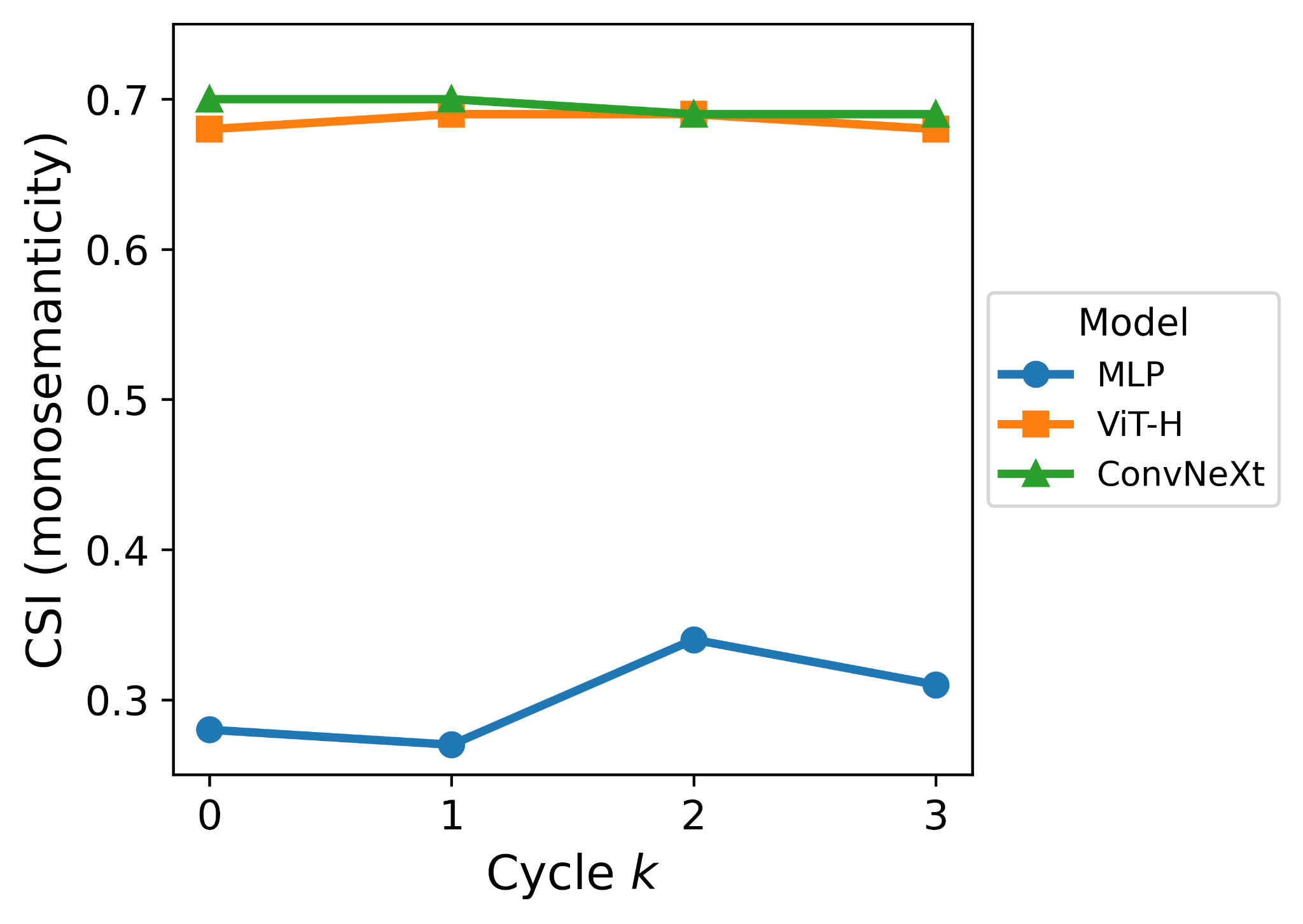
It should be noted that for ViT-H and ConvNeXt-V2 SAE-ception was applied on the final layers, which might explain why monosemanticity remains largely unchanged for these two models, as there might not be any room to "change the model's mind" at this point since features are already so well formed at this point.
This is opposed to targeting the first layer of the shallow MLP, where we do see improved monosemanticity, so perhaps we can get similar results if we target ealier layers in larger models. The final layers were chosen for ViT-H and ConvNeXt-V2 as this is much cheaper for fine-tuning.
Next Steps
While these results are neat, there still are some unanswered questions for SAE-ception. The first is can it work on LLMs and even more serious models? Additionally, there are some concerns about the quality of the SAEs across cycles, in particular feature absorption. Moreover, further experiments are needed to validate these encouraging, but small sample results.
Additionally, many optimization questions exist for SAE-ception. What is the optimal layer (or layers) to target? What is the optimal top-k for Feature Sharpening? Is our SAE based on Towards Monosemanticity good enough, or do we need a better SAE (e.g. a top-k SAE might be more reasonable for this exploraiton) for more serious versions of this method?
SAE-ception 2.0 is currently addressing the points above - the aim is to have a follow up paper ready for ICLR. Also, this code-base is so much better than the hacky first iteration (sometimes if it ain't broke don't fix it, but also, it's nice to be organized).
I'll leave it here for this brief update. More to come on other work that has occurred in the past few months. DMs are always open - please feel free to reach out regarding any questions, ideas, and/or collaboration!